A better way to make your spreadsheets readable.

My earlier post discussed how to make grid lines visible when printing a Numbers spreadsheet. The idea is to make it more readable. Here is a better way to do that while making your printed out put more visually appealing.

---

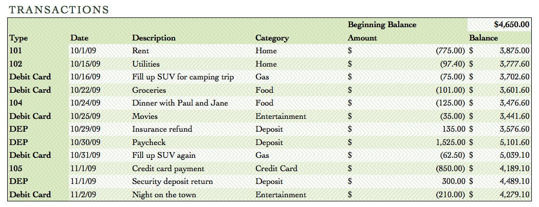
Here's a nice looking spreadsheet that has no grid lines, yet is (arguably) easily viewable. This is accomplished by alternating the colors of the rows in the spreadsheet so the eye can quickly move across the line to the appropriate column/amount. While this does take a step or two more than just making gridlines show up, it makes for a more visually appealing output when distributing your spreadsheet to other users. Here's how to do this.

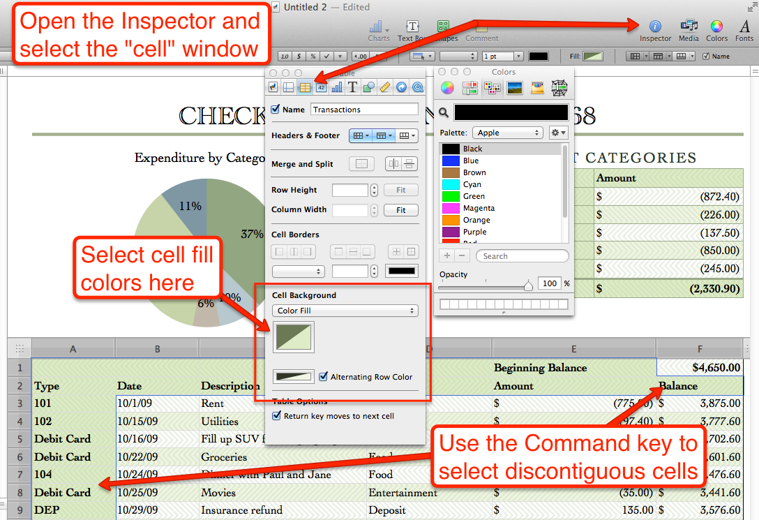
You will need to open the Inspector and find the "cells" icon like you did when making the grid lines visible. However, now, you're going to be working with cell fill colors. So the FIRST thing you need to do is select the cells that you want. In most cases you will be selecting cells that may or may no be close together. In order to select the top two rows and the first column, I had to click and drag from cell A1 to cell E2. Then, holding down the Command key, I clicked on cell F2 and then clicked and dragged from cell A3 to the bottom of the spreadsheet.

Now when I look at the color picker I can set the cell fill color to whatever I want just by clicking on the box under "Cell Background" -- "Color Fill"

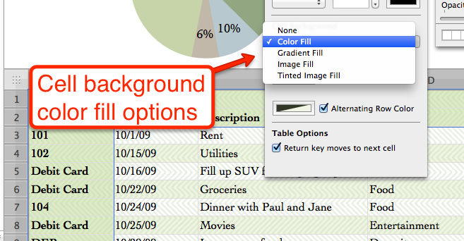I also have more options than just "Color Fill". I can use a gradient or an image or tiled image. While not that advanced, these options are better addressed in a future post. But the point is that you can creatively design your spreadsheet so that the presentation of dry, sterile information can have some snap and pazzazz!